
A Conversational AI Chatbot is Helping New Mothers Keep Healthy (#3)
Research in Translation

Introduction
Welcome back to ‘From the Computer to the Clinic’ - a newsletter about computational biology and its contributions to biomedical research.
In this newsletter, we explore how computational biology research can drive clinical progress. By sharing success stories in one disease area or domain of research, we aim to inspire the use of these successful approaches for other diseases and research areas also.
If you haven’t already, you can subscribe to this newsletter, or share it with friends and colleagues
Part III
This is part III of this series - if you missed parts I and II, you can find them on the home page of this newsletter.
An artificial neural network distills down the principles of its biological counterpart into mathematical equations – and just as the body learns to respond effectively to its surroundings, an artificial neural network can learn to perform computational tasks quite well.
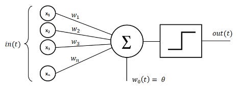
The basic unit of an artificial neural network is the perceptron. A perceptron is a lot like an individual neuron in the brain with all its connections: a number of inputs feed into a single node (the neuron), and each of these inputs has a different weight that determines its influence. At the node, these inputs (multiplied by their weights) are summed together. Mathematically, you can represent a perceptron (almost) like this:
N = w1x1 + w2x2 + w3x3 + … + wnxn
Usually, there is one more term that is added onto the sum, called the bias term (b). With the addition of the bias term, the final equation looks like:
N = w1x1 + w2x2 + w3x3 + … + wnxn + b.
The final weighted sum, bias term included, is fed into an ‘activation function’, which plays the role of deciding whether the combined inputs are strong enough to induce a response (reflecting the idea that a biological neuron only fires when the total stimulus acting on it is strong enough). A common activation function is the ReLU function, which takes any sum less than 0 and makes the output 0, and for any sum greater than 0, spits out an output equal to the sum. For example, if N = -5 in the equation above, the output will be 0 after the ReLU activation function is applied. If N = 5, the output will be 5.
The bias term is important in the context of the activation function because it can effectively amplify the input if it is set to a large enough positive value. In other words, a positive bias term means the activation function is more likely to return a non-zero value. The bias term can also dampen the input, if set to a large enough negative value, making it much harder for the activation function to return a positive input. After the activation function is applied, the final output will be passed on as input to the next layer of the neural network.
In a biological context, external information (e.g., the temperature, someone’s voice, the color of a flower) is perceived by sensory organs (temperature receptors in the skin, the ears, the eyes) and relayed along a chain of neurons to the appropriate region of the brain, which decides that it is cold, that a certain person is speaking, or that you have seen a certain variety of flower. An artificial neural network is similar - information flows into the network through the first ‘input layer’, then passes through one or more internal hidden layers where the mathematical operations described above are applied, and finally arrives at the ‘output layer’ where some decision is made. Each layer in the neural network is made up of many individual perceptrons.
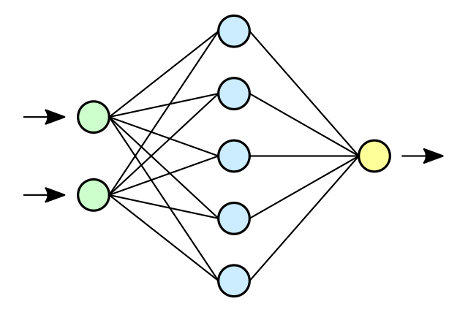
When someone talks about the architecture of a neural network, they are usually describing the layering of perceptrons (the number of layers, the number of perceptrons in each layer, etc.), and how these layers are connected. A very common way to arrange perceptrons inside a neural network is as a ‘fully connected’ layer (you can see an example of this in the figure below): each of the neurons in the input layer are connected to all of the neurons in the next layer, and each these connections (there will be N x M connections, where N is the number of neurons in the input layer and M the number of neurons in the internal, ‘hidden’ layer) has its own weight.
The idea of setting up the network in this way is that each neuron in the middle layer will capture some pattern of interest from the input layer that depends on a unique combination of input neurons. The more neurons you have in the second layer, the more of these patterns the network can potentially detect and take into account when making a decision.
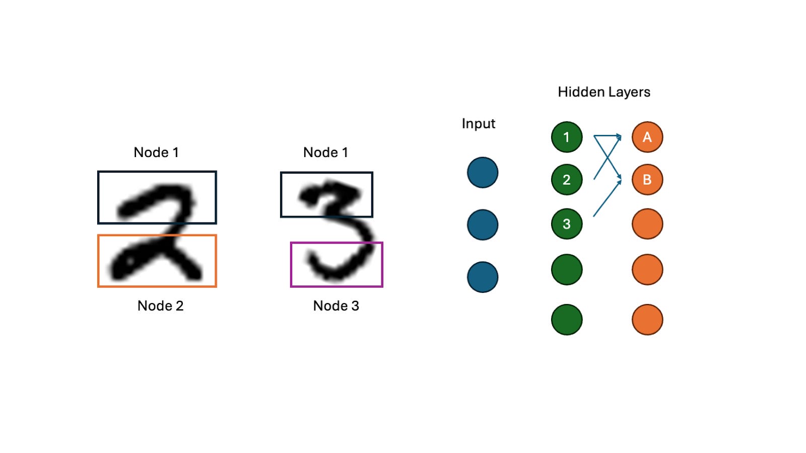
To provide even more pattern-detecting power, many neural networks are constructed with multiple hidden layers inside of the network between the input and the output layer. These networks with multiple internal layers are called deep neural networks (the process of training these networks to perform useful tasks is called deep learning), and they can detect hierarchical patterns.
A classic example that illustrates these ideas is the problem of recognizing hand-drawn numbers (is this number a one, a two, a three?). The first hidden layer in the neural network might recognize basic fragments or motifs in these images - for example, the arc at the top of the numbers 2 and 3. The next layer in the network can detect combinations of these basic motifs, and the next layer combinations of these combinations, and so on, such that the output layer receives a final report about what combinations of motifs are present in the image and use this information to decide what number it has been presented with.
This layering and connecting of perceptrons with many different weights is what makes neural networks such a powerful tool. They can pick up on complex patterns in input data (sets of images, patient clinical data, etc.) that humans observing the data would have a hard time seeing, and then make decisions based on the complex patterns they detect.
What does it mean for a neural network to make a decision? Typically, a network is either classifying something (taking an input image and deciding whether it is a dog or a cat, deciding whether someone has a disease or not given their clinical data, etc.) or it is performing a task called regression, meaning that it is predicting an output value based on a set of input values. An example of a regression problem is predicting the average rent price of a 3-bedroom apartment in a city given factors like median income, the rate of construction, etc.
One final important point about neural networks: where do the weight and bias terms we’ve been discussing come from? How are their values determined? This is an important question because it is ultimately the values of these ‘parameters’ that give a neural network its power to address a specific challenge. A neural network trained to distinguish images of cats from dogs may have exactly the same architecture (same number of layers, same number of nodes per layer, etc.) as one that is designed to distinguish cars from tractors, but the two networks will not have the same parameters.
Initially, when setting up a neural network, it is common to set all the weight and biases to random values. You then give the neural network training data, and ask it to perform a chosen task (some form of classification or regression). At first, it will perform terribly. Like asking a very young child who has never seen an animal before to tell you if the new pet you brought home is a cat or a dog, an untrained neural network trying to classify images of dogs and cats will just make random guesses. But as it sees more and more training data, and is told when it guesses wrongly, the neural network will progressively update its parameters (the weight and bias terms) until it gets very good at classifying dogs and cats correctly. How these adjustments are made involves some more complex math, and I won’t dwell on it here, but there are many good videos (including this series) that explain it well if you want to learn more.
Stay tuned for part IV…